Interpretation & inversion

We interpret data for subsurface anomalies and changes, we match data to the response from models and invert for reservoir density and density changes and for subsurface compaction.
Picture showing gravity and depth changes (subsidence) above a gas accumulation.

Gravity and depth changes (subsidence) above a gas accumulation. Values are proportional to the area of the circles. Blue means increase and red decrease. To the right is a cross-plot of gravity change and subsidence. Below is a sketch of the gas accumulation, gas production from a nearby gas reservoir and likely movements of fluid contacts. From (Eiken et al. 2023).

Subsurface insights: Time-lapse gravity data interpretation

Time-lapse gravity data can be more straightforward to interpret than most other geophysical data. This is because the signal is proportional to mass changes, which are fundamental to understand the dynamics of the subsurface. It does not rely on complex rock physics relations, as seismic and CSEM data do. Microgravity can be powerful when flowing fluids have large density contrasts, such as gas–water and air–water. Also, injection or extraction with the related pressure changes cause expansion or compression in a reservoir, which can result in measurable surface gravity changes.

Height changes may have many different causes and can be interpreted in terms of subsurface rock strain. This again is the result of pressure changes and rock compressibilities.

Model matching

A further stage of data analysis is to compare observations with models of changes in gravity or height. This is a way of identifying surprises, and may initiate model updates. Model matching can be done in Attrack‘s time-lapse module.

The Chi squared sum (Χ2) statistic is useful for parameter fitting and history matching of observed vs. modelled changes (following Vevatne et al., 2012):

where N is the number of seafloor stations, ΔzR is the measured relative depth change, c1 is a data offset (to be fitted), c2 is a scale factor (to be fitted), Sm is modelled subsidence, and σ is the estimated error of a measured difference.

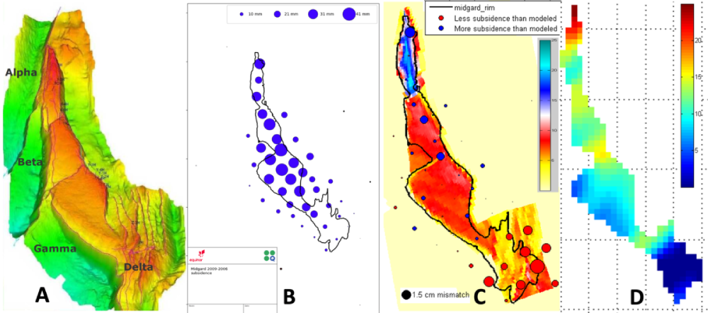
The figure below show in (B) seafloor subsidence of up to 4 cm over 3 years at the Midgard field (Eiken et al. 2022). Panel C shows the mismatch with the subsidence predicted from the reservoir flow model coupled with a Geertsma geomechanical model, for each station. The red circles in the south (the Delta-segment) show that the seafloor has subsided less than expected. A well was drilled into the Delta-segment and received water breakthrough already after two years of production. The subsidence mis-match suggested faults acted as barriers. A new well was drilled and confirmed the lack of depletion.

 
Picture of graph showing depth map of midgard field.

A: Depth map of the Midgard field with warm colors as shallow and green as deeper, showing the main fault segments, B: 2009-2006 subsidence shown as circles with radius proportional to the value C: Difference between observed and modelled subsidence. Backdrop colors show modelled compaction (in cm), and the circle radius is proportional to the subsidence mismatch. Red circles mean the observed subsidence is less than modelled. D: Inversion for reservoir compaction (in cm) using a Geertsma geomechanical model of the overburden. From Eiken et al. (2022).

Picture shows a woman working on her computer with time-lapse data.

Time-lapse data

Inversion

Time-lapse data may be inverted for reservoir changes with reservoir geometry as constraint. Gravity data are inverted for density and height change data for strain (vertical compaction). From these, fluid and pressure changes may be inferred. Subsidence maps can be inverted for lateral variation in reservoir pressure and rock compressibility (e.g. Fokker et al. 2012), which again can identify undrained compartments in a producing oil or gas field. Inversions can also be useful for identifying anomalous (and possibly erroneous) stations in a densely sampled grid.

Inversion of either mass changes or vertical compaction/extension is in Attrack done by Tikhonov regularization. The number of stations is less (or much less) than the number of cells in the reservoir model. Inversions will have a much larger number of unknows than number of equations, and the (unconstrained) problem is ill-posed. This is also due to the smoothing effect of Newton’s law. The solution is stabilized by the Tikhonov smoothing parameter, and further constrained by the reservoir top and bottom bounding surfaces, within which changes can occur. The minimum and maximum value allowed in each cell can be limited by the user.

Tikhonov linear inversion of the subsidence data at Midgard (D in the figure above) clearly indicated the location of a sealing fault.

Contact us for onshore & offshore solutions

Get in touch with us